In this post, we will discover how to construct a classifier utilizing a basic Convolution Neural Network which can categorize the images of client’s xray to spot wheather the client is Regular or impacted by Pneumonia.
To get more understanding, follow the actions appropriately.
Importing Libraries
The libraries we will utilizing are:
- Pandas- The pandas library is a popular open-source information control and analysis tool in Python. It offers an information structure called a DataFrame, which resembles a spreadsheet or a SQL table, and permits simple control and analysis of information.
- Numpy- NumPy is a popular open-source library in Python for clinical computing, particularly for dealing with mathematical information. It offers tools for dealing with big, multi-dimensional varieties and matrices, and provides a wide variety of mathematical functions for carrying out operations on these varieties.
- Matplotlib- It is a popular open-source information visualization library in Python. It offers a variety of tools for developing top quality visualizations of information, consisting of line plots, scatter plots, bar plots, pie charts, and more.
- TensorFlow- TensorFlow is a popular open-source library in Python for structure and training maker discovering designs. It was established by Google and is commonly utilized in both academic community and market for a range of applications, consisting of image and speech acknowledgment, natural language processing, and suggestion systems.
Python3
|
|
Importing Dataset
To run the note pad in the regional system. The dataset can be downloaded from[ https://www.kaggle.com/datasets/paultimothymooney/chest-xray-pneumonia ] The dataset remains in the format of a zip file. So to import and after that unzip it, by running the below code.
Python3
|
|
Check out the image dataset
In this area, we will attempt to comprehend imagine some images which have actually been offered to us to construct the classifier for each class.
Let’s load the training image
Python3
|
|
Output:
['PNEUMONIA', 'NORMAL']
This reveals that, there are 2 classes that we have here i.e. Regular and Pneumonia.
Python3
|
|
Output:
There are 3875 pictures of pneumonia imfected in training dataset . There are 1341 typical images in training dataset
Plot the Pneumonia contaminated Chest X-ray images
Python3
|
|
Output:
.png)
Pneumonia contaminated Chest X-ray images
Plot the Regular Chest X-ray images
Python3
|
|
Output:
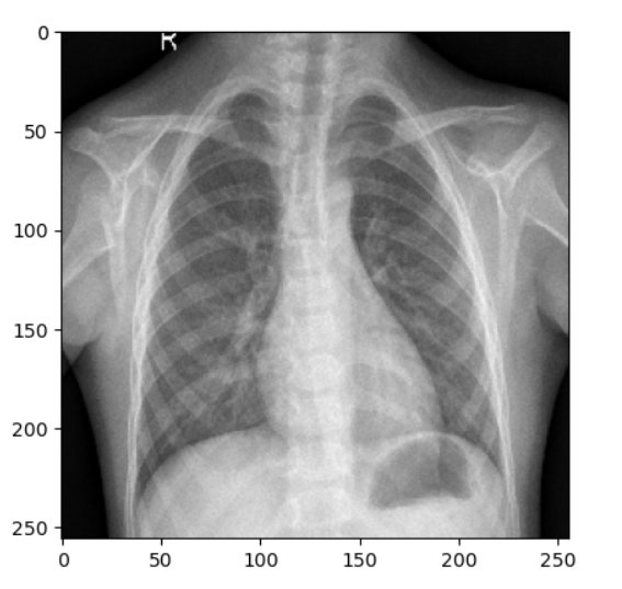
.png)
Regular Chest X-ray images
Information Preparation for Training
In this area, we will categorize the dataset into train, test and recognition format.
Python3
|
|
Output:
Found 5216 files coming from 2 classes. . Found 624 files coming from 2 classes. . Discovered 16 files coming from 2 classes.
Design Architecture
The design architecture can be referred to as follows:
- Input layer: Conv2D layer with 32 filters, 3 Ã 3 kernel size, ‘relu’ activation function, and input shape of (256, 256, 3)
- MaxPooling2D layer with 2 Ã 2 swimming pool size
- Conv2D layer with 64 filters, 3 Ã 3 kernel size, ‘relu’ activation function
- MaxPooling2D layer with 2 Ã 2 swimming pool size
- Conv2D layer with 64 filters, 3 Ã 3 kernel size, ‘relu’ activation function
- MaxPooling2D layer with 2 Ã 2 swimming pool size
- Conv2D layer with 64 filters, 3 Ã 3 kernel size, ‘relu’ activation function
- MaxPooling2D layer with 2 Ã 2 swimming pool size
- Flatten layer
- Thick layer with 512 nerve cells, ‘relu’ activation function
- BatchNormalization layer
- Thick layer with 512 nerve cells, ‘relu’ activation function
- Dropout layer with a rate of 0.1
- BatchNormalization layer
- Thick layer with 512 nerve cells, ‘relu’ activation function
- Dropout layer with a rate of 0.2
- BatchNormalization layer
- Thick layer with 512 nerve cells, ‘relu’ activation function
- Dropout layer with a rate of 0.2
- BatchNormalization layer
- Output layer: Thick layer with 2 nerve cells and ‘sigmoid’ activation function, representing the possibilities of the 2 classes (pneumonia or typical)
In summary our design has:
- 4 Convolutional Layers followed by MaxPooling Layers.
- Then One Flatten layer to get and flatten the output of the convolutional layer.
- Then we will have 3 completely linked layers followed by the output of the flattened layer.
- We have actually consisted of some BatchNormalization layers to allow steady and quick training and a Dropout layer prior to the last layer to prevent any possibility of overfitting.
- The last layer is the output layer which has the activation function sigmoid to categorize the outcomes into 2 classes( i, e Regular or Pneumonia).
Python3
|
|
Print the summary of the design architecture:
Output:
 Design: "consecutive"

. _________________________________________________________________
. Layer (type) Output Forming Param #

.=============================================================
=
===
. conv2d (Conv2D) (None
,

254, 254, 32) 896
.
. max_pooling2d (MaxPooling2D( None, 127, 127, 32)
0


.)
.
. conv2d_1( Conv2D )( None
,

125, 125, 64) 18496
.
. max_pooling2d_1 (MaxPooling (None, 62,
62, 64
)

0

. 2D)
.
. conv2d_2( Conv2D)( None
,

60,
60, 64) 36928
.
. max_pooling2d_2 (MaxPooling (None, 30,
30, 64
)

0

. 2D)
.
. conv2d_3( Conv2D) (None
,

28, 28, 64) 36928
.
. max_pooling2d_3 (MaxPooling( None, 14, 14, 64
)
0


. 2D)
.
.

flatten (Flatten) (None, 12544) 0
.


. thick (Thick) (None
,
512)
6423040
.

. batch_normalization (BatchN( None, 512) 2048
.
ormalization)
.
.

dense_1(
Thick)( None, 512) 262656
.
. dropout( Dropout)(
None, 512)
0


.
. batch_normalization_1 (Batc( None, 512) 2048
.
hNormalization)
.
.

dense_2(
Thick)( None, 512) 262656
.
. dropout_1( Dropout)(
None, 512)
0


.
. batch_normalization_2 (Batc( None, 512) 2048
.
hNormalization)
.
.

dense_3(
Thick)( None, 512) 262656
.
. dropout_2( Dropout) (None
,
512)
0


.
. batch_normalization_3 (Batc( None, 512) 2048
.

hNormalization)

.
. dense_4( Thick)( None, 2) 1026
.
.===============================
=
===== ======= =========
=
========= ==
.
Overall params: 7,313,474
.
Trainable params: 7,309,378
. Non-trainable params: 4,096
. _________________________________________________________________
The input image we have actually taken at first resized into 256 X 256. And later on it changed into the binary category worth.
Plot the design architecture:
Python3
|
|
Output:
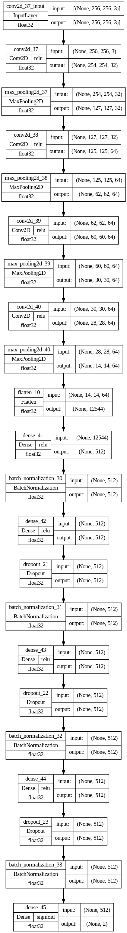
Design
Assemble the Design:
Python3
|
|
Train the design
Now we can train our design, here we specify dates = 10, however you can carry out hyperparameter tuning for much better outcomes.
Python3
|
|
Output:
 Date 1/10

. 163/163 [==============================] - 59s 259ms/step - loss: 0.2657 - precision: 0.9128 - val_loss: 2.1434 -val_accuracy: 0.5625
.
Date 2/10
. 163/163[==============================] - 34s 201ms/step - loss: 0.1493 - precision: 0.9505 - val_loss: 3.0297 -val_accuracy: 0.6250
.
Date 3/10
. 163/163[==============================] - 34s 198ms/step - loss: 0.1107 - precision: 0.9626 - val_loss: 0.5933 -val_accuracy: 0.7500
.
Date 4/10
. 163/163[==============================] - 33s 197ms/step - loss: 0.0992 - precision: 0.9640 - val_loss: 0.3691 -val_accuracy: 0.8125
.
Date 5/10
. 163/163[==============================] - 34s 202ms/step - loss: 0.0968 - precision: 0.9651 - val_loss: 3.5919 -val_accuracy: 0.5000
.
Date 6/10
. 163/163[==============================] - 34s 199ms/step - loss: 0.1012 - precision: 0.9653 - val_loss: 3.8678 -val_accuracy: 0.5000
.
Date 7/10
. 163/163[==============================] - 34s 198ms/step - loss: 0.1026 - precision: 0.9613 - val_loss: 3.2006 -val_accuracy: 0.5625
.
Date 8/10
. 163/163[==============================] - 35s 204ms/step - loss: 0.0785 - precision: 0.9701 - val_loss: 1.7824 -val_accuracy: 0.5000
.
Date 9/10
. 163/163[==============================] - 34s 198ms/step - loss: 0.0717 - precision: 0.9745 - val_loss: 3.3485 -val_accuracy: 0.5625
.
Date 10/10
. 163/163 [==============================] - 35s 200ms/step - loss: 0.0699 - precision: 0.9770 - val_loss: 0.5788 - val_accuracy: 0.6250
Design Assessment
Let’s imagine the training and recognition precision with each date.
Python3
|
|
Output:
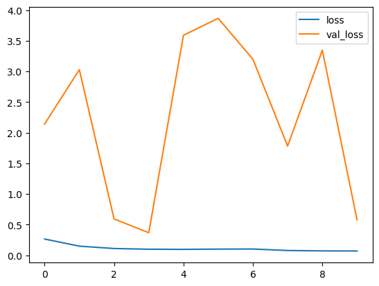
Losses per models
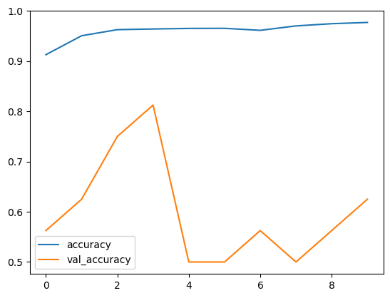
Precision per models
Our design is carrying out great on training dataset, however not on test dataset. So, this holds true of overfitting. This might be because of imbalanced dataset.
Discover the precision on Test Datasets
Python3
|
|
Output:
20/20 [==============================] - fours 130ms/step - loss: 0.4542 - precision: 0.8237 . The precision of the design on test dataset is 82.0
Forecast
Let’s examine the design for random images.
Python3
|
|
Output:
 1/1 [==============================] - 0s 328ms/step

.
Pneumonia
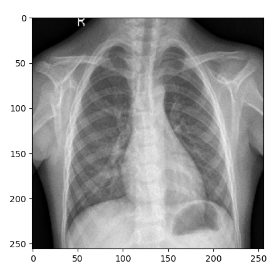
Regular Chest X-ray
Python3
|
|
Output:
1/1 [==============================] - 0s 328ms/step . Pneumonia
Pneumonia Contaminated Chest
Conclusions:
Our design is carrying out well however according to losses and precision curve per models. It is overfitting. This might be because of the out of balance dataset. By stabilizing the dataset with an equivalent variety of typical and pneumonia images. We can get a much better outcome.